A new table should be created in a new sheet. Although it is possible to add a new table in an existing sheet, it tends to be difficult to see the tables.
(Note) As mentioned before, sheets are called "tables" in StarSuite Calc. Be careful not to get confused.

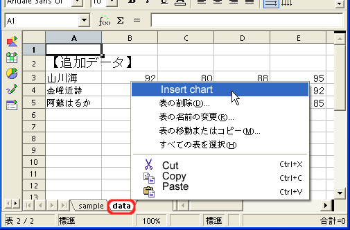
Sheets can be inserted by right-clicking on the "Sheet Index Tab", selecting "Insert Table" next, and clicking "OK" in the dialog which appears next. In the dialog, you can specify the position to insert the new sheet, and name the new sheet. (These settings can be changed after the sheet is created.)

Let's add a new sheet.
Click the sheet index tab named "Data" to display the sheet, right-click on the sheet tab "Data" and select "Insert Table".


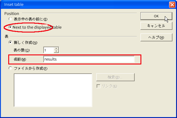
In the dialog that appears next, check the "Next to the displayed table" as the insert position, write "Results" as the sheet name, and click the "OK" button.


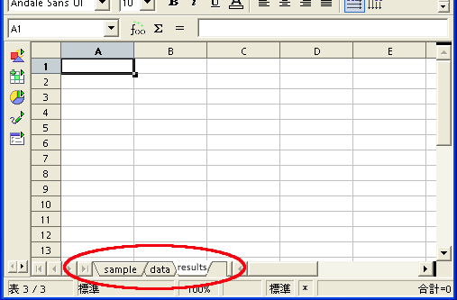
A new sheet (table) named "Results" has now been created.

Data (a cell or a range of cells) in a sheet can be utilized from other sheets by referencing them.

How to do that is exactly the same as when they are on the same sheet. The only difference is that you have to select the target sheet by clicking the sheet index tab when specifying the reference (a cell or a range of cells) in a formula. While you are writing a formula, the active cell remains active even if you display a different sheet.

Let's summarize the results of the calculations of the sheet "Sample" in the sheet "Results" you have just created.

Input text as follows in the new sheet "Results".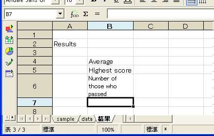


Let's display the average of the total scores in cell C4.
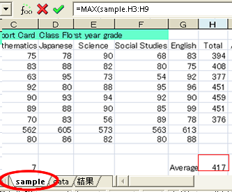
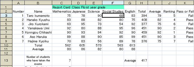
Since the average of the total scores has already been obtained in cell H13 of the sheet "Sample", all we have to do is reference the cell from cell C4. However, in cell H13 of the sheet "Sample", the property of the cell has been changed so as not to display decimal fractions. If the data is referenced without this specification, the decimal fraction will be displayed in C4. Although we can set the same property for C4 as cell H13 of the sheet "Sample", let's use the round function explained above to display the score as an integer.

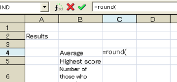
After activating cell C4, input "=round(".


Then, click the sheet index tab "Sample" and cell H13 that contains the average of the total score.


The average score was chosen. Click the sheet index tab of the sheet "Results" and go back to the original sheet. Since cell C4 is still active, the formula "=round(sample.H13" is being displayed as in the following illustration.


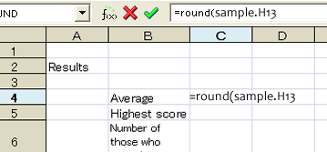
The designation "sample.H13" means cell H13 of the sheet "Sample". The cell address that we have been using is effective only in the same sheet, and it is a rule to add the sheet name with " " after this when a cell is referenced from other sheets.
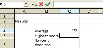
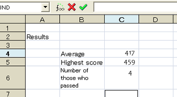
Now, press the Enter key to set the formula. The average score of 417 will be displayed in cell C4 as in the following illustration.

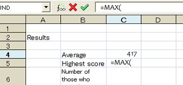
Let's display the highest score in cell C5 next.
The highest score was mentioned as an example in the explanation of the general functions. It can be obtained using the function "max", which obtains the highest value.
After inputting "=max(" in cell C5,


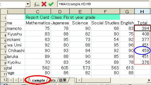
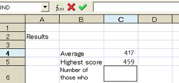
drag the mouse from cell H3 to H9 in the sheet "Sample", and press the Enter key. Then the window automatically goes back to the sheet "Results", and "C5" will be set. In C5, the highest score of 459 will be displayed.


Let's display next the number of those who passed in cell C6.
Since the decision to pass or fail is also performed in column K of the sheet "Sample", you have only to count the number of those who passed. The function that is useful in such a situation is "countif".

The function "countif" has the following features.

• If a cell range is specified as the first argument and a condition is specified as the second argument, the number of the data that meet the conditions is displayed.

Since the first argument is the object of the condition specified as the second argument, the left-hand side (target) of the formula is omitted unlike in the normal conditional expression. Since the format is uncompleted, it is surrounded by "" (double quotation marks). (e.g. ">100")

Let's practice the function in cell C6.
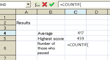
Input "=countif(" in cell C6,


drag the mouse from cell K3 to K9 in the sheet "Sample",


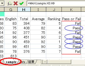
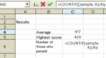
and go back to the sheet "Results" by clicking its tab. The screen should look like the following illustration.


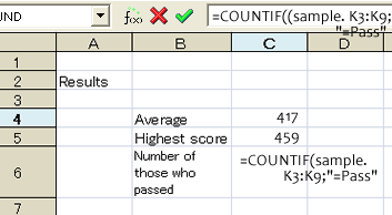
(In order to count the number of columns that contain the text "pass"), input [;"=pass"] at the end of the formula and press the Enter key. Then, the number of those who passed, 4, will be displayed.


Finally, let's display the graph in the sheet "Results", too.
Display the sheet "Sample", click the graph that you created, cut the graph by holding down the Ctrl key and pressing the x key (or right-click the mouse on the graph and select "Cut"), go back to the sheet "Results", and paste the graph by holding down the Ctrl key and pressing the v key (or right-click on the graph and select "Paste"). Adjust the layout of the graph by changing its position and resizing it for better viewability.


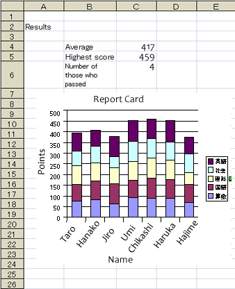
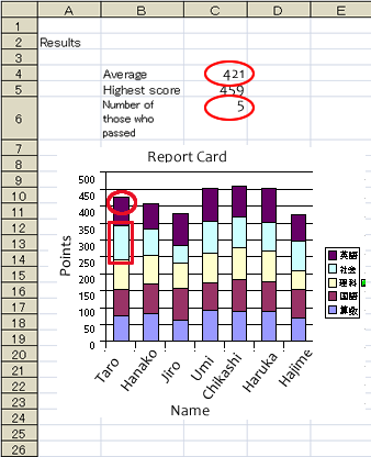
Now the sheet "Results" is completed! When you are not interested in the individual data and want to know only the general results, this sheet is more convenient since it is simple and easy to see.

By the way, this sheet references the sheet "Sample". What happens if the source data is changed?
Let's change Taro Kumamoto's score for social studies from 68 to 100 as a trial, and see what happens.

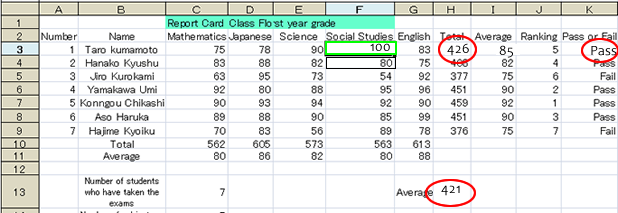
The average of total scores increased (417 -->421). In addition, since the total score for Mr. Kumamoto exceeded 400, his status was changed to "pass". Accordingly, the number of those who passed changed to 5.
Then, display the sheet "Results". You can see that the above changes are reflected in the sheet "Results", including in the graph.