This section is a continuation of the explanation of the “Auto-fill of Formulas” and “Average Score of Each Subject” which was suspended in section 3.5 “Utilizing Useful Functions and Features”.

In the section 3.5, “Utilizing Useful Functions and Features”, we experienced that formulas were easily copied with the auto-fill feature. When formulas were copied with the auto-fill feature (or with the normal copy and paste feature), the referenced ranges were automatically adjusted as we intended.

This is because spreadsheets have a function to reference cells according to the relative positional relation to the cell specified in the formulas 、 when handling formulas. This function is called the “relative reference” of cells.

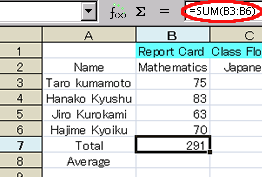
For example, the formula “=SUM(B3:B6)” written in cell B7 is interpreted, when copied, as

• “get the total value from the cell in the same column and 4 cells above (B3’s relative position from B7) to the cell on the same column and 1 cell above (B6’s relative position from B7) seen from the cell in which this formula is written (B7).”

Accordingly, when this formula is copied and pasted using the auto-fill feature, each pasted formula conveys the meaning:

• “Get the total of the values from the cell in the same column and 4 cells above to the cell in the same column and 1 cell above seen from the cell in which this formula is written”,

and the formulas are automatically written as we intend.

This function is very useful. Once a formula is written, even if it is complicated, all you have to do is copy it when the same calculation is required in other rows or columns. Thus, repeating the same calculation is easy even in large tables.

Although the “relative reference” is very useful, it does not always work well.

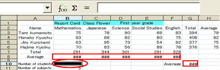
One such example is getting the average score for each subject.
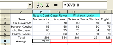
It seems that the average score for each subject can be obtained using the following process, since we already have the total scores for each subject and the number of the examinees.

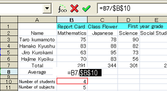
1. Display the average score for mathematics in B8 cell by dividing B7, which is the total of the scores for mathematics of all the examinees, by B10 which is the number of the examinees and pressing Enter.





2. Then, activate cell B8 and drag the auto-fill handle to F8. The average of each subject seems to be obtained like this.

However, as you can see from the result, errors occur in auto-filled cells. (The result is the same even if the data are copied and pasted.) Why?

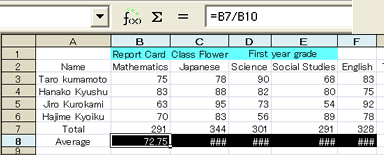
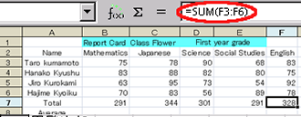
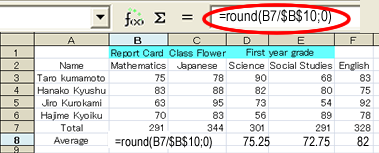
To find out the reason, look at the formula written in the cell F8. It looks like the figure below.

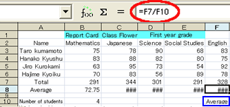
As for the numerator, there is no problem since it is F7 which contains the total scores for English, but something is wrong with the denominator. It should be B10 which is the number of examinees, but was changed to F10. (This creates a formula that divides a numeric value 328 by a text “Average”, and obviously an error has occurred.)

Think it over carefully. As explained in the previous section, “Cells are referenced by a relative reference when formulas are copied.” So this is the natural result.

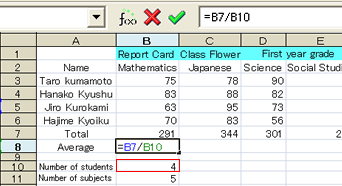
In the source cell, B8, “=B7/B10” is written.

That means the formula commanding

• “Divide the cell in the same column and 1 cell above (B7) by the cell on the same column and 2 cells below (B10) the cell in which this formula is written (B8).”

was copied.
Thus, the formula copied to F8 is commanding;

• “Divide the cell in the same column and 1 cell above (F7) by the cell in the same column and 2 cells below (F10) the cell in which this formula is written (F8).”

So this is working correctly.
However, the average of each subject cannot be obtained this way.

This problem occurs because 、

• the denominators of all formulas should reference B10 which contains the number of examinees, but the address of the referenced cell is automatically changed due to the relative reference function.

In applications other than spreadsheets, automatic calculations are not performed even if a formula is copied and this kind of problem does not occur.

This means that, generally speaking,

• the problem will be solved, if we can stop the automatic calculation of referenced cells and copy the same cells when a formula is copied.

The “absolute reference” is the feature that meets this requirement.
This is a function to reference the absolute position that has no relation to the cell position in which the formula is written instead of referencing the relative position from the cell in which it is written when a formula references cells.

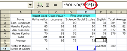
To set an “absolute reference” in a formula, put the $ symbol in front of the row number and column number of the cell address, as in “$B$10”, instead of “B10”.
In StarSuite Calc, switching to absolute reference can be performed by holding down the Shift key and pressing the F4 key instead of directly adding $.

Let’s obtain the average score for each subject using this function now.

To make things clear, delete what you wrote before first.

To delete data in a cell,
  select the target to delete cell and perform one of the following actions.

• Press the Back Space key.
• Hold down the Ctrl key and press the X key.
• Right-click the mouse and select “Cut”.
• Press the Delete key, select “Delete all” and click on “OK”.
• Right-click the mouse and select “Delete contents”. Then, select “Delete all” and click on “OK”.

Drag the mouse and select the range from B8 to F8, and delete the data using one of the above actions.

These cells have now been cleaned up. Now follow the instructions below.

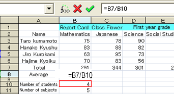
1. Input “=” in cell B8, click the cell B7 which contains the total score for mathematics of all the students, input the division operator “/”, and click the cell B10 which contains the number of examinees. So far, this is the same as before.





2. While B10 is selected, hold down the Shift key and press the F4 key.By doing this, B10 changes to $B$10 which specifies an absolute reference. Then set the formula.
(Note) If you press the F4 key more than one time by mistake, one or both of the $ marks may disappear. In such a case, press F4 some more times and the formula returns to the correct format.





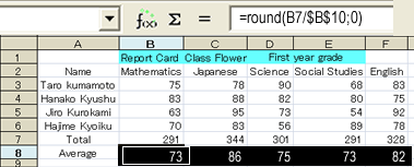
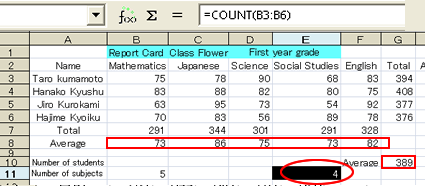
3. Finally, activate cell B8 and drag the auto-fill handle to F8. Now the average of the scores for each subject is being displayed.。

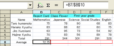
The average score of each subject was obtained using the above procedure.
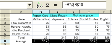
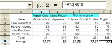
To confirm if the formulas were copied correctly, look at F8. You can see that a formula to divide the total score of English (F7) by the number of examinees (B8) is there.

Why don’t we display these average scores as whole numbers as we did in section 3.5 “Utilizing Useful Functions and Features”. In section 3.5, we changed the property of the cells. This time, we will use a new function called “ round”.

The function “round”works as below.

• By inputting a value to be displayed as the first argument of the function, and the number of decimals as the second argument, the display format of the values is changed.

Since we want to display values as whole numbers here, the number of decimals should be 0.

Thus, activate cell B8,
input “=round(B8/$B$10;0)”, and set the formula. Then, copy the cell B8 to the cells from C8 to F8 using the auto-fill feature. The task is now completed.

Let’s use this opportunity to obtain each examinee’s average score per subject in column H using the same method as above.

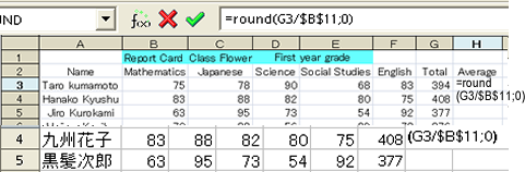
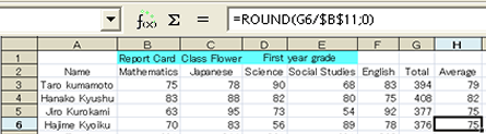
In cell H6, Hajime Kyoiku’s average score per subject is being displayed. Cell H6 contains a formula that divides his total score, G6, by B11 and rounds the result to a whole number.


(Note) If you do not copy a formula, you do not have to worry about the “relative reference” or “absolute reference”. The same cell is referenced no matter whether or not the $ mark is added.

(Note) When you copy formulas with the auto-fill or the Copy & Paste feature, be sure to check some of the copied formulas. If they are not copied as you intend, consider whether “absolute reference” can solve the problem.

(Note) “Relative reference” and “absolute reference” are distinguished only when formulas are copied. After Copy & Paste is finished, there is no difference between “relative reference” and “absolute reference”. (More precisely, “if the cell is not copied and pasted again, then whether there is a “relative reference” or “absolute reference” makes no difference.)

For example, cell B10 which displays the number of examinees is cut (by holding down the Ctrl key and pressing X), and pasted into cell E11 right afterwards (by holding down the Ctrl key and pressing V).

When cell B10 is cut, an error occurs in the cells that display the average score for each subject. However, after the data in B10 is pasted to another cell, the calculation is performed correctly as before.
For confirmation, look at the formula in cell F8, and you can see that the denominator remains an “absolute reference”, but the cell address is automatically changed as we intend.