In spreadsheets, formulas that reference any cells are re-calculated automatically each time the contents of some of the cells are changed (regardless of whether or not the formulas reference the cells whose contents have changed).

For example, if the cell B3 (Taro Kumamoto’s score for mathematics) is changed from 75 points to 80 points, three cells other than B3 are automatically changed as below.

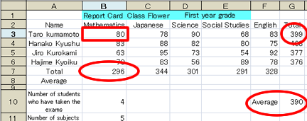
Since the contents of the cell B3 were changed, all formulas were re-calculated and the values in the three cells that referenced (utilized) cell B3 were corrected.
Since the automated re-calculation is executed in cells that contain formulas each time the data or formulas are revised, in spreadsheets, as just described, we can change the data and formulas as often as we like. It’s just too much work to do this with a handwritten table and a calculator, isn’t it?

(Note) However, it is inconvenient if re-calculation is executed every time data is input when you are creating a large table since it is necessary to wait while the re-calculation is being done. In such cases, you can stop automatic re-calculation by selecting “Cell Contents” from the “Tool” menu and un-checking “Automatic Calculation”. Note that you have to remember to execute the re-calculation manually as required. Otherwise, the results of the calculation will be shown wrongly. (Select “Re-calculation” in the “Automatic Calculation” mentioned above, and the re-calculation is executed.)

Let’s insert a blank row as described below.
Before this, change the value in cell B3 that you changed in the previous section back to 75. (You can do this by holding down the Ctrl key and pressing the z key.)

Row and column insertion is generally executed as follows.

1. Click on the row (or column) number next to where you want to insert an additional row (or column), and select the whole row (or column).
2. Right-click somewhere on the row (or column) number field.
3. Select “Row Insertion” (or “Column Insertion”).

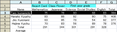
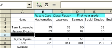
Insert a new row just above the line for Taro Kumamoto.

1. Select row 3 by clicking on the row number “3”.





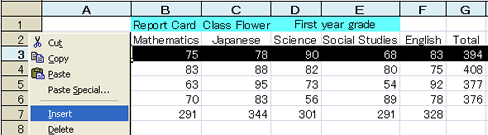
2. Right-click somewhere on the row number field and select “Row Insertion”.





3. A blank row is then inserted.

By doing this, the row numbers of row 3 and the following rows increase by one.
For example, the cell address in which Taro Kumamoto’s mathematics score (75 points) is input changes as follows.

• Before insertion → B3
• After insertion → B4

Don’t you think this causes a problem?
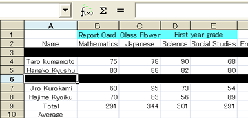
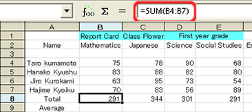
For confirmation, the final status of last week is shown below.

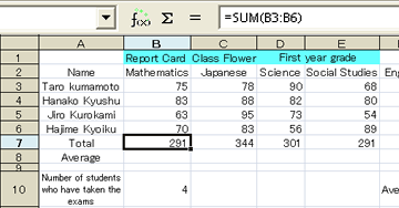
For example, to obtain the total score for mathematics, the following formula was input in cell B7 as the above figure.

    ＝ＳＵＭ（Ｂ３：Ｂ６）
  (Although all letters are written in double-byte here to facilitate visualization, actually they need to be written in single-byte letters.)

Since this formula calculates the total value from cell B3 to B6, it became necessary to change the cell range after an additional row is inserted at the position of row 3. To be concrete, we need to change the above formula to

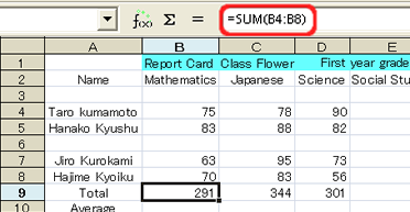
    ＝ＳＵＭ（Ｂ４：Ｂ７）

to obtain the total score for mathematics. It is troublesome to re-write formulas all the time.

In spreadsheets, however, when rows or columns are inserted or deleted, referenced cell addresses in formulas are automatically calculated and adjusted as we specify them.

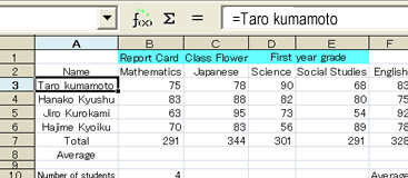
Activate cell B8 after a row has been inserted, and you can see this as in the following figure.

Isn’t it smart?

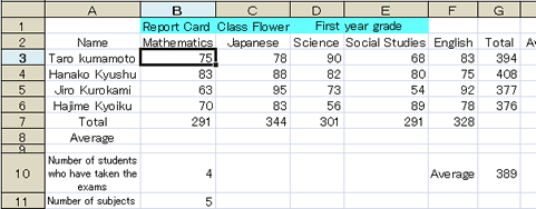
Next, insert another row above Jiro Kurokami.

This time again, the formula in cell B9 which displays (calculates) the total score for mathematics was correctly adjusted to include the inserted row as in the following figure.

Like this, spreadsheets have a function to automatically adjust the cell numbers to maintain referenced cells in formulas as they are specified, even if additional rows or columns are inserted. I think you can understand how user-friendly spreadsheets are.

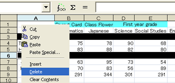
At the end of this section, delete the inserted two rows and return the table to its original state.

To delete rows or columns, the following steps are generally taken.

1. Click the row (or column) number that you want to delete to select the whole row (or column).
2. Right-click on somewhere in the row (or column) number field.
3. Select “Delete Rows” (or “Delete Column”).

To select more than one row that are not adjacent each other and delete them at one time, hold down the Ctrl key and click on the numbers of the target rows (or columns). Then, you can select multiple lines.

Specifically, follow the instructions below.

1. Hold down the Ctrl key, 、 and click on the numbers for rows 3 and 6.
If you select the wrong row by mistake, select the row number again to clear your selection.




2. Right-click on somewhere in the row number field, and select “Delete Rows”.





3. The table has now been restored to its former state.