| Managing Rows and Columns |
Practice operations related to rows and columns such as the insertion of row data or column data, changing the width, etc.
Inserting Rows/Columns
Let’s expand the table by adding data prepared in another sheet.
Spreadsheets consist of multiple independent sheets like presentation software or drawing software. Sheets (In StarSuite Calc, this sheet is sometimes called a "table") are switched by clicking on the "Sheet Index Tab" at the bottom of the screen.
Click the "Sheet Index Tab" on which "Data" is written, and display the second sheet.
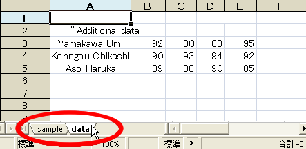
In this sheet, data is stored for 3 examinees to add to the other sheet. So let’s insert this data into the first sheet.
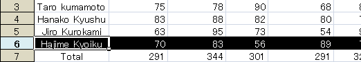
Drag the mouse from row number 3 to 5 to select the rows, right-click the mouse, and select "Copy". (You can hold down the Ctrl key and press C key instead.)
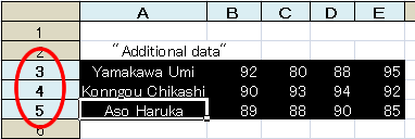

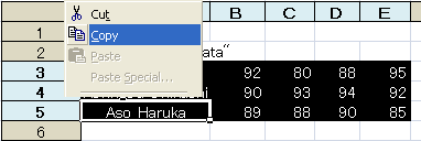
By doing this, data on 3 examinees was copied.
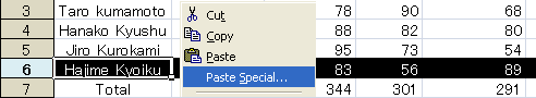
Copy this data on top of Hajime Kyoiku’s data in the first sheet. To do this, click the "Sheet Index Tab" on which "Sample" is written to display the first sheet and click on row number 6 to select Hajime Kyoiku’s data.
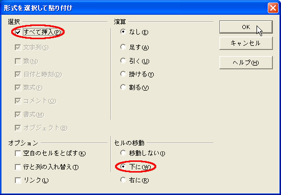
Right-click the mouse and select "Paste specifying format", then, the dialog below appears.
Check "Insert All" in the "Select" field, and "Downward" in the "Move of cells", then click "OK".
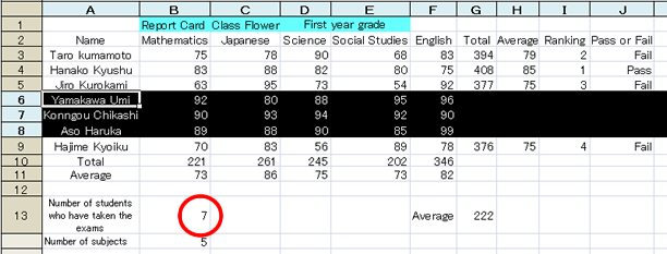
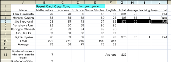
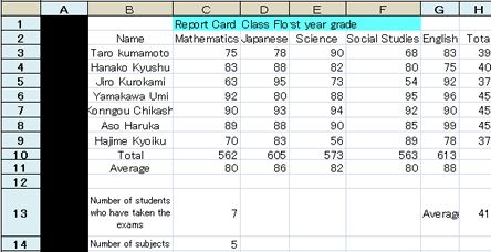
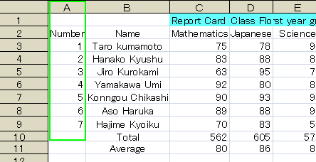
The data for 3 examinees is thus inserted into the table as below.
Note that the number of examinees was automatically changed to "7". (The automatic calculation feature of spreadsheets is really useful, isn't it?)
The total score and the average score of each subject (B10, B11, etc.) also include the scores of the 7 examinees. Check this if you have time.
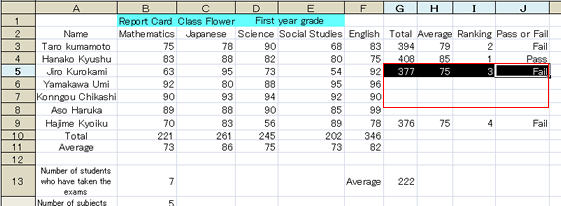
The individual' s total scores and average scores still remains blank. So copy the formulas to these cells using the auto-fill feature.
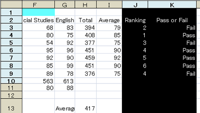
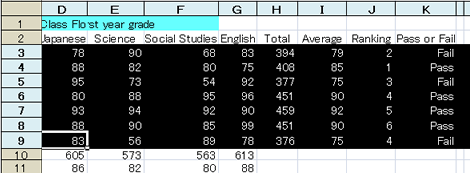
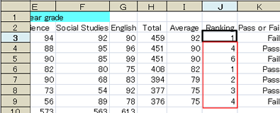
Select from G5 to J5 at one time and drag the auto-fill handle down to 3 rows below. The data for the 3 examinees that were added is completed.
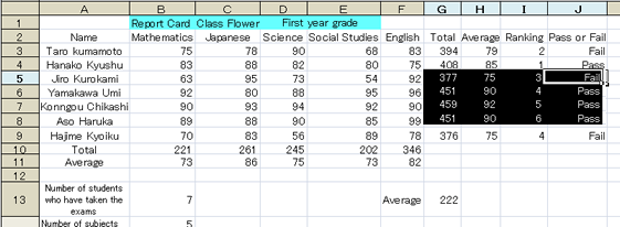
Not only is the ranking out of order, there are two fourth places. This is because "3" in cell "I5" was simply copied with the auto-fill feature. To rank them correctly, it is necessary to sort the data by the total score of each examinee and rank them as we did in section 3.6, "Sorting and Judging by the Conditions". We will do this at the end of this section.
Changing the Row Width and Column Width
When you want to change the size of a cell, change the row width or column width that includes the cell.
To change the row width or column width,just drag the frame of the row number field or the column number field.
To change the width of multiple rows or columns at one time,
select the rows and columns whose width you want to change, and drag the frame of one of the selected row numbers or column numbers.
In preparation for the next section, insert some blank columns and adjust their width.
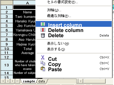
Click the column number (alphabet) "A" to select column A.
Right-click the mouse and select "Insert Columns" to insert a column to the left of the column A.
Then, drag the border line between the inserted column A and column B, and narrow the column width to the approximate size in which two double-byte characters can fit.
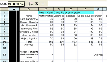
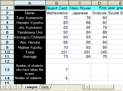
In preparation for the next section, input the text "Number" in cell A2. If the column width is not appropriate, adjust it again.
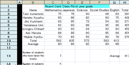
Then, input the number "1" in cell A3, auto-fill the cells down to A9 to number the cells. You did it correctly if your table looks like the following.
Change the width of column J and K at the same time.
Drag the mouse from column number J to K to select the two columns, narrow their width to the approximate size in which two double-byte characters can fit by dragging the right line of the frame of the column number J or K.
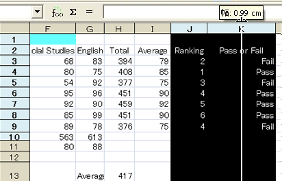
By doing this, the width of column J and K can be narrowed in the same width at once.
Let’s correct the ranking next. This is a review of section 3.6, "Sorting and Judging by using Conditions".
Select the rows from row 3 to row 9 to be sorted. (Drag the mouse from row number 3 to 9.)
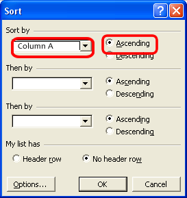
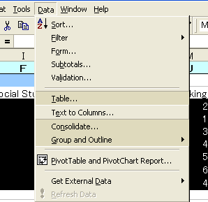
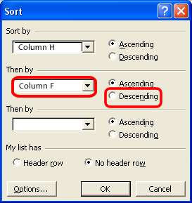
Select "Sort" from "Data" menu.
The key should be column H and the sorting order should be descending, right?
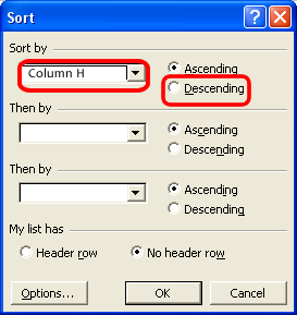
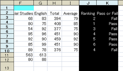
However, if there are the same scores in the column H, the ranking will be underspecified with this setting alone. In fact, both of the total scores of row 4 and row 5 (column H) are 451 in the above table. When there is a possibility of such a case, set the "second preference key" in sorting the data. In the following example, column F (the score for social studies) is specified as the "second preference key". Then, if there are the same values in the first preference key, the second preference key is used to determine the order.
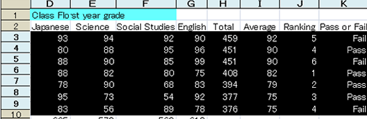
In the above example, since the score for social studies of row 5 is higher than that of row 4, the ranking did not change.
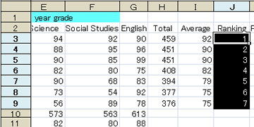
Correct the number in the top cell of the ranking (J3) to "1", and auto-fill the following cells.
Finally, sort the data by the examinee number. Select the rows from row 3 to row 9 to be sorted. (Drag the mouse from the row number 3 to 9.), and select “Sort” from the “Data” menu. Specify column A which contains examinee numbers as a key and ascending as the sorting order.