
| Inputting and Editing Data |
Master how to input and edit data in a spreadsheet StarSuite Calc (Table Calculation Document).
Inputting Data (Texts and Numbers) in StarSuite Calc
Input texts and numbers as you like into the ex1.sxc which you saved in Practice 5.
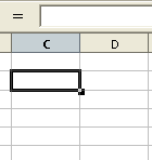
To input data (texts and numbers), select a cell where you want to input data to make it active (subject of the operation). (The active cell is surrounded by a bold black border.)
Input the text or numbers from your keyboard. The text or numbers will be inserted into the active cell. At the same time, the text or numbers you are inputting are displayed in the formula bar.


When you finish inputting the data (text and numbers) that you want to insert into the cell, press either the Enter (Return) key, TAB key, or Arrow keys to set the input data.
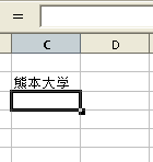
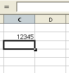
Text data is then aligned to the left and numbers-only data is aligned to the right as above. At the same time, the active cell moves. (In the above example, it moved down.)
(Note) When you set the input, the direction of the movement of the active cell varies depending on the key you press, as follows. These keys can be used not only when you want to set your input, but at any time you want to move the active cell.- Enter key : The active cell moves downward. (Hold down the Shift key and press Enter to move the active cell upwards.)
- TAB key : The active cell moves to the right. (Hold down the Shift key and press TAB to move the active cell to the left.)
- Arrow keys : The active cell moves in the direction of the selected arrow key.
When you want to input double-byte numbers-only data, select “Cell” from the “Format” menu, then select “Text” under “Number” tab, and input the data.
Changing the Data (Texts and Numbers) of StarSuite Calc
Revise (change) the texts and numbers you have entered into ex1.sxc in Practice 6 as you like.
(1) Change data in the Formula Input Box (This method is common.)
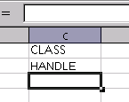
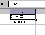
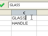
(Example) Change “CLASS” in the cell C1 to “GLASS”
Click on the cell whose data you want to change and make it the active cell.

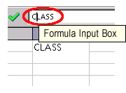
Change the content of the cell displayed in the Formula Input Box.
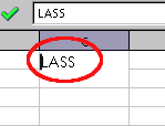
When you finish, press Enter to set the change.
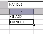
You can see that the data of cell C1 has been changed to “GLASS” and the active cell has moved to C2.
(2) Directly change the data in the cell(Example) Change “GLASS” in the cell C1 to “CLASS” again.
Double click on the cell whose data you want to change.
Change the data directly in the cell whose data you want to change.
When you finish, press Enter to set the change.
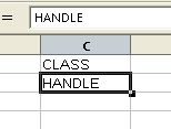
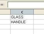
You can see that the data of the cell C1 has been changed to “CLASS” and the active cell has moved to C2.
Range Selection of Cells
Select a cell, a row, a column, or a random range using the cells of ex1.sxc you input/changed texts and numbers in Practices 6 and 7.
When you copy or move data or set a format for text, select the target cell or range first. If you select multiple cells, rows or columns, all cells are effected by these operations at one time.
- Selecting a cell
Click on a cell. (Make it active). - Selecting rows and columns
Click on the row number or the column number.


- Selecting the whole sheet
Click the cross point of the row numbers and column numbers in the upper left corner.

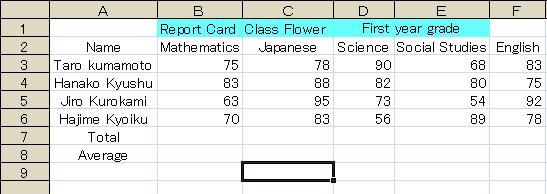
- Selecting a cell range
(Method 1)
Press the left mouse button on the starting cell and drag it to the ending cell of the range you want to select.
(Method 2)
Click the starting cell of the range you want to select and then click the ending cell while holding down the Shift key.


(Note) Multiple rows and columns can be selected using the same method as above.

Changing the Method of Displaying the Characters (Changing a Cell Property)
Change cell properties (text, background, ruling, etc.) as you like using the data you input into ex1.sxc in Practice 6, etc.
The display method of the input data can be changed by cell. That is because each cell has various properties such as the font type, font size as well as the display method for numbers, background color, frames (ruling), etc.
These properties can be set from “Cell” under the “Format” menu after you select the cell or the range of cells.、
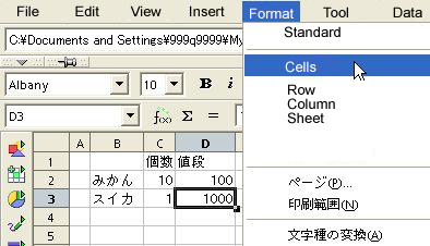
- Regarding numbers (values), you can change the number of decimals, the display format for dates and times, etc. by selecting the “Numbers” tab.

For example, if you select the display method for currencies as above, the displayed value changes as below.


(Note) In a spreadsheet, the numeric data (numbers) are usually treated as calculable “values”. They are aligned to the right. If you want to input numbers as text numbers, put a single-byte single quote symbol in front of the numbers as in “’1234”. You can use this method when you want to enter numbers as double-byte characters.
In the following example, the number of oranges (cell C2) has been changed to a “text number.” You can see that the “text numbers” are aligned to the left.


- The background color can be set by selecting the “Background” tab.

The following is an example of the use of different background colors for the cell. (The background color for the orange and watermelon has been changed.)

- Since the sheets of a spreadsheet consist of cells, it looks as though there are lines (rulings) between the cells. However, these lines are not necessarily printed. In order to display and print these rulings, you need to change the settings from the “Frame” tab.
Select “Ruling position” and choose the line width. It is also possible to display only the lines required and change the width of each line from the “User Definition” settings if necessary.

If cell D3 is set as above, the result is as shown below. A line is drawn only at the bottom of the cell.


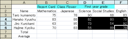
When you choose a range of cells, you can draw a line either around the range or around each cell of the range.

The following is an example of a line drawn around a range. The settings are as above.


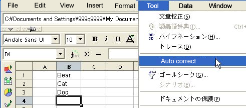
By default (a state in which no settings have been changed), when alphabetic characters are input, he first letter is automatically converted into a capital letter.
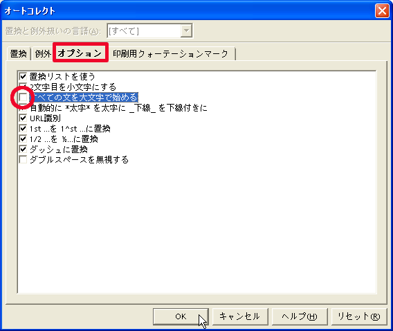
To cancel this setting, select “Autocorrect” from the “Tool” menu, uncheck the “Start all sentences with caps”, and click “OK”. This setting affects the whole sheet, and not only a cell or a range of cells.
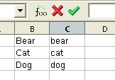
Even if you change this setting, the method of displaying letters that have already changed to capital letters will not be affected. After you change the setting, the first letters of sentences will remain as they were input. In the following example, after data was input in column B, “Start all sentences with caps” under “Autocorrect” was unchecked, and other data was input into column C with lower-case letters. You can see that each word in column C starts with a lower-case letter.
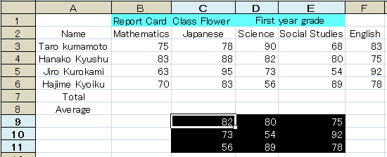
Copying and Moving Data
Try out the edit functions such as Copy, Paste, and Move in the ex1.sxc with which you set the format in Practice 9.
Like other software, the input data can be copied using Copy & Paste. 。
Select a cell range first, and copy using one of the following methods.
- Select “Copy” from the “Edit” menu.
- Hold down the “Ctrl” key and press the “C” key.
- Select “Copy” after clicking the right mouse button somewhere within the selected range.
Click the upper left cell of the range where you want to paste the data.
Finally, paste the copied data using one of the following methods.
- Select “Paste” from the “Edit” menu.
- Hold down the “Ctrl” key and press the “V” key.
- Select “Paste” after clicking the right mouse button on the selected cell.択
If you want to move a range instead of copying it, you can drag the range directly using the mouse.
Inputting a Series of Data
Try out the input function for a series of data using ex1.sxc that you used in Practice 10.
(Since this is a very convenient function, it is important to master it.)
By using the “Autofill” function, you can copy data or input a series of data by increasing or decreasing them according to fixed value.
You can configure the detailed settings for the input function for a series of data from “Series of Data” under the “Edit” menu.
- Copying text using the autofill function
Place the mouse pointer on the black square (autofill handle) in the lower right corner of the active cell (the shape of the mouse pointer changes to “+”) and drag the autofill handle (along the row or column direction only, and not in the oblique direction).
Then the same text is copied into each of the cells selected by dragging.


- Inputting numbers while increasing them by one using the autofill function
Drag the autofill handle of a cell with a number input. Then the numbers are input increasing by one into the cells selected by dragging.


(Note) If you want to input (copy) the same number (not increasing them), hold down the “Ctrl” key while dragging the autofill handle.


-
Inputting numbers while increasing them by a fixed value using the autofill function
Select consecutive two cells in which numeric data has been input, and drag the autofill handle. The cells across which the mouse was dragged will be populated with numbers increasing by the difference between the two initial cells.


- Inputting a series of text data
In addition to numbers, you can create a custom list of sequential data. Select “Option” from the “Tool” menu, and then “Sequential List” under “Table Calculation Document”. Some lists are already registered. An example using the days of the week is shown below.


