Let’s practice some often-used functions and useful features.

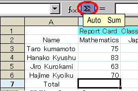
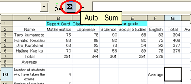
The icon “Σ” on the Formula Bar is called the “AutoSum Button”. The total of the adjacent rows or columns can be obtained by just clicking this icon.
The reason why only the “SUM” function has an icon out of the hundreds of functions prepared is that it is the most frequently utilized function.

As an example, obtain the total scores for mathematics using the “AutoSum button” in preparation for obtaining the average by subject later.

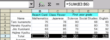
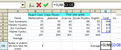
1. Click and activate cell B7, and click on the “Σ (AutoSum button)”.





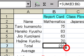
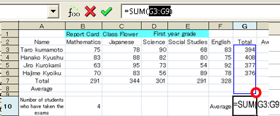
2. Then, “=SUM()” is automatically input without inputting “=”, and the adjacent cell range that contains the numeric data is selected at the same time. (In this case, the outline of the selected range turns blue.)
   If the selected range is correct, just press Enter. If the selected range is not correct, drag the black square on the lower right of the selected range to select the correct range and press the Enter key.
   
   
   
   
   That’s it! Isn’t it easy?
   
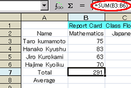
   For confirmation, click and activate cell B7. The desired “=SUM(B3:B6)” is displayed in the Formula Input Box.
   
   
   
   
   

Inputting a calculation formula becomes even easier if you apply the “autofill” feature that copies the same data or populates increasing or decreasing data into cells for the calculation formulas.

Let’s obtain the total score for each subject using the “autofill” feature.

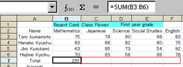
1. Click and activate cell B7 in which the total score for mathematics was input in the previous section.





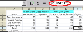
2. Drag the autofill handle (the black square in the lower right corner of the cell) to cell F7.。






That’s it! Isn’t it easy?

For those who are wondering if the formula was correctly input, let’s confirm it. Click and activate cell F7. You can see the desired “=SUM(F3:F6)” is displayed in the Formula Input Box. The formula was input correctly.




(*) Suspicious you, (That is a university student. Excellent!) try other cells, too.

The reason why the formulas referencing different cells are created by copying with the autofill feature like this is explained in section “3.8 Referencing Cells”.

In a large spreadsheet, it is difficult to count the number of the data on the screen. Even if the number of data is not many, you have to re-count them each time you insert (add) or delete data.
Leave such mechanical work to the PC.

The count function undertakes this task. It counts and outputs the number of numeric data included in arguments. If the argument is a range selector (cell addresses divided by “:” (colon)), the number of the data contained in the range is output.
Formulas are also treated as numeric data as long as the calculation result (output) is numeric data.

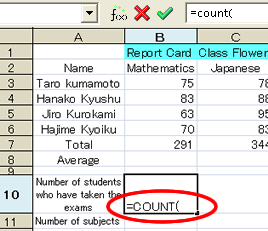
Let’s count the number of examinees and display it in cell B10.

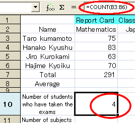
1. Click and activate cell B10 and input “=count(”.





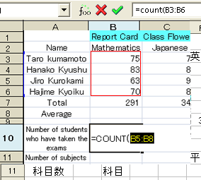
2. Drag the mouse from B3 to B6. The range is selected and “B3:B6” is specified as the argument of the count function.





3. Press Enter to complete the input. Since the number of examinees is four (consisting of four lines of data), the number 4 should be displayed in cell B10.
   Click and activate cell B10 and you can see that the formula of the count function is displayed in the Formula Input Box.

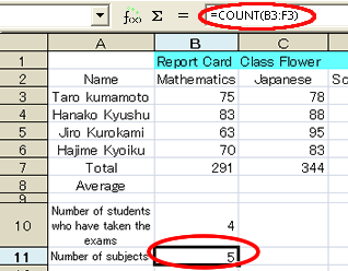
You can display the number of subjects using the same method (selecting someone’s scores for all subjects) in cell B11 as follows.
For example, select the range from B3 to F3 and use the count function.

In order to display the average of the total scores in cell G10, you need to divide the grand total of the student’s total scores by the number of students in cell B10.

1. Activate cell G10 first and click the AutoSum button.






2. Since unnecessary cells are included, drag the black square on the lower-right corner of the selected area and re-select the correct area. Now, the grand total of the student’s total scores can be calculated.









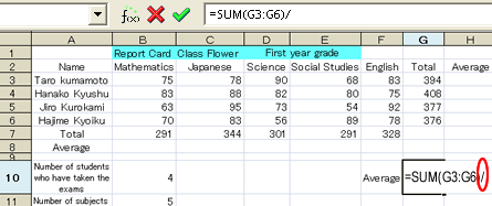
3. Then, input the division operator “/” after that.





4. Click cell B10 and press Enter to complete the formula.

At this point, the symbols “###” appear in cell G10. These symbols indicate the fact that the value in the cell cannot be displayed since the cell width is too narrow. In the example here, the result of the division had a decimal point and the number of digits to be displayed increased. The number “388.75” displayed in the lower right corner of the window is the result of the calculation. Space for six digits is required to display this value in the cell including the decimal point.

Although the value can be displayed without generating the “###” error symbol, if you expand the cell, there is no point in displaying the average score in such detail. So, let’s…

• Round the result to a whole number so that it is displayed in the cell.

From “Format” menu, select “Cell” → “Number” tab → “Classification” → “Numeric Value” → “Format” → [-1234], and click OK.

(Note) [-1234] specifies the format that “displays only the integer part”.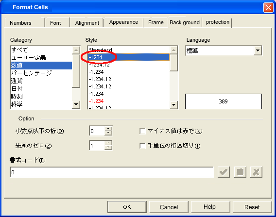

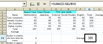
Now, the average score is being displayed as a whole number as follows.

(Note) Actually, a function named average () is available to obtain averages. With this function, you can obtain averages more easily. Try it yourself.

(Note) Even if the result of the calculation is being displayed as a whole number by changing the format, the information on the fractional part is kept (as internal information) in the program.

(Note) Regarding the average by subject, additional explanation is required. It will be mentioned in section “3.8 Referencing Cells”. Please look out for it.