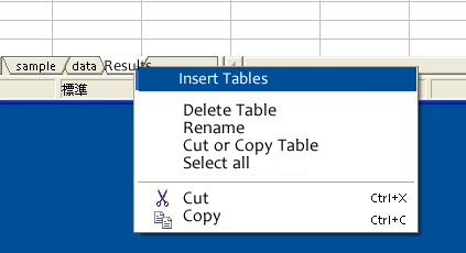
A sheet can be inserted into the file you are creating from other calc files. You can do this by right-clicking the mouse on a "Sheet Index Tab", selecting "Insert Tables", and clicking "OK" in the dialog that appears next.

Let's add the sheets of the file you have just downloaded next to the sheet "Results". Display the sheet "Results" by clicking its Sheet Index Tab, right-click the mouse on the tab, and select "Insert Tables".

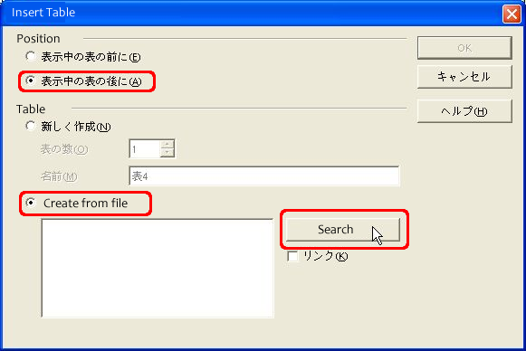
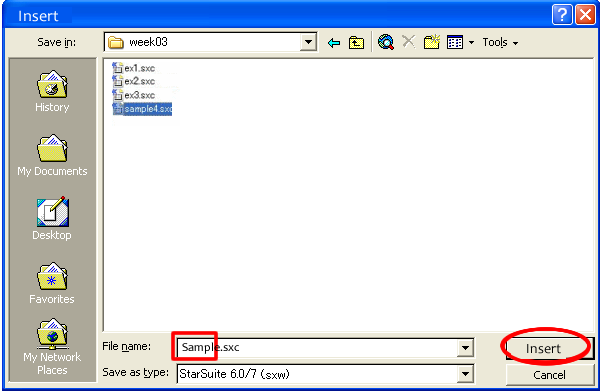
In the dialog that appears next, check "Next to the displayed table (A)" and "Create from file (F)", press the button "Search", select the file sample.sxc that you have just downloaded and click the button "Insert".




Select the required sheets from the displayed titles of the sheets in the sample.sxc file.
This time, we will use all the sheets. So hold down the Shift key and select the two sheet names and press the button "OK".



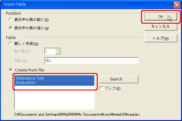
Now, the sheets "Attendance Test" and "Evaluation," were added next to the sheet "Results".

In the sheet "Attendance Test", students' attendance at each lecture of a certain class (6 times) and the results of three times taking tests are input. "1" represents attendance and "0" represents absence. The tests are on a 100-point scale.

The conditions for pass or fail and for point additions are as follows.

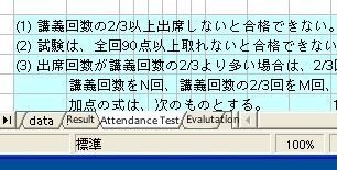
  (1) Attendance at two-thirds or more of all the lectures is required to pass.
  (2) It is necessary to get more than 90 points (out of 100 points) in each test to pass. 
  (3) If a student attends two-thirds or more of all lectures, he or she gets additional points depending on the number of times attendance exceeds two-thirds of the lectures.
       Points to be added are calculated by the following formula in which the number of all lectures is represented by N, two-thirds of the number of lectures is represented by M, and the number of attendances is represented by L.
           10*(L-M)/(N-M)  (The maximum number of points to be added is 10.)
  (4) If the total score of a student exceeds the total of the passing scores, points will be added depending on the score. The points to be added are calculated by the following formula in which the total of the perfect scores is represented by I, the total of the passing scores is represented by J, and the total score of the student is represented by K.
          30*(K-J)/(I-J)  (The maximum number of points to be added is 30.)

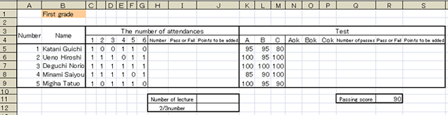
Input formulas that obtain the following items in the columns under "Attendance".

• Number of Times": The number of attendances (Use the function "countif".)
• "Pass or Fail": Pass or fail according to the conditions on attendance specified above. Display "pass" if a student satisfies the condition, otherwise display "fail". (Use the function "if".)
• "Points to Be Added": Points calculated by the formula specified as a condition above
• Number of Lectures": The number of all lectures (Use the function "count".)
• "2/3 Number": Two thirds of the number of all lectures (Pass line on attendance)

   (Note) Be sure to reference the cell that contains the "2/3 Number" in the formula for "Points to Be Added."

Input the formulas that obtain the following items in the columns under "Tests".

• "Aok": Pass or fail on the test A. Display "1" for pass, and "0" for fail. (Use the function "if".)
• "Bok", "Cok": Same as "Aok"
• "Number of Passes": Number of times a student achieved a passing score out of three times taking the test. (Use the function "countif".)
• "Pass or Fail": Pass or fail according to the conditions on the test specified above. Display "pass" if a student satisfies the condition, otherwise display "fail". (Use the function "if".)
• "Points to Be Added": Points calculated by the formula specified as a condition above

   (Note) Be sure to reference the cell that contains the "Passing Score" in the formula of "Points to Be Added."

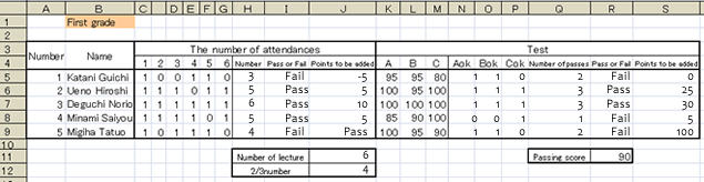
The result of inputting the above formulas will look almost like the following illustration. However, some mistakes are included in the following illustration on purpose. If your table looks exactly like this, it means the formulas you have input are wrong.

Input formulas in the sheet "Evaluation".

• In the "Number" field, display the data in the number field in the sheet "Attendance Test" as it is.
• In the "Name" field, input the student's last name and first name leaving one space (a single-byte space) between them. (Refer to the Utilization of the Character String Conjunction Operator "&" near the end of this page.)
• With regard to the "Performance" field, follow the instructions below. (Refer to the Utilization of the Logic Operator "AND" near the end of this page.)


• If the number of attendances is higher than two-thirds of the number of all lectures and all of the test scores reached the passing score, display a score obtained by the following formula.
        60 + Additional Points on Attendance (max. 10) + Additional Points on the Tests (max. 30)
  
• Otherwise, display "failure".

The result of inputting the above formulas will look almost like the following illustration. However, some mistakes are included in the following illustration on purpose. If your table looks exactly like this, it means the formulas you have input are wrong.

(Note 1) Utilization of the Character String Conjunction Operator "&"
   When you want to connect character strings (sets of characters), use the operator "&".
For example, to connect three character strings, "999q9999", "@", and "st.kumamoto-u.ac.jp", write the formula
The character strings are connected and make one character string.
If you want to leave a space between the two character strings to be connected, put a space character " " (there is a blank space in the middle of the double quote).
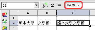
For example, if you want to leave a space between the university name and the department name in connecting "Kumamoto University" and "Literature Department", it will work well if you input as follows.

If you just connect "Kumamoto University" and "Literature Department", the connection will turn out as follows.




(Note 2) Utilization of the Logic Operator "AND"
   When there are multiple conditions, they can be combined in various ways.
When there are multiple conditions, they can be combined in various ways.

1. If it rains and is cold, I will wear my coat.
2. If it rains or is cold, I will wear my coat.

Although these conditional expressions are based on two conditional factors "it is raining" and "it is cold", satisfying the both conditional factors is the ultimate condition in the first sentence, and satisfying either one of those conditional factors is the ultimate condition in the second sentence.   The combination of conditions expressed with "and" like the first sentence is generally called an "AND(operation)", and the combination of conditions expressed with "or" like the second sentence is generally called an "OR(operation)."
   In StarSuite Calc, these operations are also defined as functions.
For example, the conditional expression that means [Cell A1 is "rain" and cell B1 is "cold"] is written as follows. Likewise, the conditional expression that means [Cell A1 is "rain" or cell B1 is "cold"] is written as follows. Now, what should we do to display "raincoat" when cell A1 is "rain" and cell B1 is "cold", and otherwise display "nothing"? We can do that by combining the function "IF" and the function "AND" as follows. The initial "=" is the symbol to start a calculation formula.
When the function AND or the function OR is used independently, "=" is necessary at the head of the formula. (e.g. =AND(A1="rain";A2="cold")) In this case, if the condition is satisfied,"TRUE" is desplayed and if the condition is not satisfied, "FALSE" is displayed in the cell.